BUS 202 Quantitative Analysis II
Solutions to Assignment 5
1.
a)Laplace     b)MaxMin    c)MaxMax    d)MinRegret
  23.5           12           35           21
  22.5           18           27           15
  25             22           28           13
  26.5           20           33           15


Regret Table:
                           Max
    0    3    3    21       21
    8    0    8    15       15
   13    0    3     5       13
   15    0    0     0       15
Laplace criterion chooses decision 4; MaxMin decision 3; MaxMax
decision
1; and MinRegret decision 3. [Any
questions?]
2.a)Laplace     b)MaxMin    c)MaxMax    d)MinRegret
  6.67            5            8           2
  6.00            6            6           3
  4.33            1            9           7


Regret Table:
                      Max
    1    2    0       2
    0    3    2       3
    3    0    7       7
Laplace criterion chooses decision 1; MaxMin decision 2;
MaxMax
decision 3; and MinRegret decision 1. [Any
questions?]
3.
- a) EMV of the four Decisions are: | 22.2| 22.3 | 25.3 | 27 |
Therefore the best decision is #4.
- b) Expected regrets are | 6.3 | 6.2 | 3.2 | 1.5 |
Therefore the best decision is again #4.
- c) Maximum Expected monetary value and Minimum expected
regret
always select
the same decision.
[go to top] [Any
questions?]
5.
- a) Accept Govt contract (min payoff is $1000 versus $-1000 for
Brochure
Job)
- b) Accept Govt Contract (EMV of the decisons are | $1000 |
$666.67|
resp)
- c) E(V) = 4000*P(J) + (-1000)*[1-P(J)]
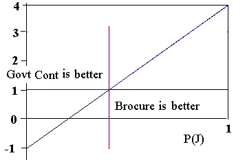
- d) P(J) = 0.4 . (for any P(J) less than 0.4 Govt Contract
has
higher EMV.)
e)
Regret Table
|
NJ |
J |
| Govt. Contract |
$0 |
$3000 |
| Brochure |
$2000 |
$0 |
Bid on Brochure ( worst regret is $2000, while it is $3000 for
Govt
Contract)
- f) Accept Govt Contract ( Expected regrets are |$1000 | $1,333.3|)
- g) EVPI= Expected value with perfect information -
Expected Value without
Perfect information
= (2/3)* $1000 + (1/3)* $4000 - $1000 (from part b above) = $1,000
- This is EVPI Expected value of perfect Information
[go to top] [Any
questions?]
6.
a)
Small:       (0 + 1000 + 2000 + 3000)/4  =  $1,500
Medium:     (-1000 + 0 + 3000 + 6000)/4  =  $2,000
Large:    (-3000 -1000 + 4000 + 8000)/4  =  $2,000
Medium and Large tie for best expected dollar return
b)Utilities of the payoffs from the graph:
Decision   Cold     Cool     Warm    Hot        E(U)
Small       .66     .73      .78     .83        .75
Medium      .55     .66      .83     .93        .7425
Large       .14     .55      .87     .98        .635
Small has the maximum expected utility. Working backwards with
the
utility graph (finding the $ value corresponding to the expected
utilities
of the alternatives) we find that "Small" has a certainity equivalent
of
about $1,800; "Medium" of about $1700 and "Large" less than $0.
[go to top] [Any
questions?]
8.
a) Equivalent lottery for a net cash flow of $0 is obtained from
p*50,000
+ (1-p)*(-20,000)= $0 solving for p gives p = .28.
Equivalent lottery for a net cash flow of $20,000 is obtained from
p*50,000 + (1-p)*(-20,000)= $20,000 solving for p gives p = .57.
b) 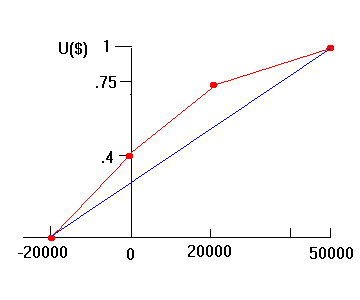 .
.
For me, the lottery of winning $50,000 or loosing $20,00 if
the probability of winning is .40 is barely worth a sure $0. Thus
my
utility of a sure $0 is 0.4 ( > .28).
Likewise the lottery of winning $50,000 or loosing $20,000 is
just about as desirable as a sure $20,000 if the winning
probability
is .75, thus my utility for a sure $20,000 is .75 (> .57).
Therefore, my utility function for money is given in red .
c)I am risk averse since my utility function is concave. To accept
a lottery (with risk) I demand a premium in the form of higher winning
probability (40% as opposed to 28% in the case of $0; and 75% as
opposed
to 57% in the case of $20,000). If I were risk indifferent my utility
function
would have been the blue line for which the utility of the lottery
with
expected value $0 and the sure $0 has the same utility.
[go to top] [Any
questions?]
10.
a)
                   .25              .75
Decision          Rainy            Sunny            E(V)
  GO            -15,000           10,000          $3,750
  CANCEL         -1,000           -1,000         $-1,000
Thus GO is the best decision
b) Expected Value (EV) with perfect information:
.25 *(-1,000) + .75 *(10,000) = $7,250
Hence: Expected Value of Perfect Information (EVPI) = 7,250 - 3,750
= 3,500
[go to top] [Any
questions?]
11.
States of nature: - Sunny: S
- Rainy: R
Result of report (Event): - Predict Sunny: PS
- Predict Rainy: PR
Priors:  P(S) = .75          P(R) = .25
Reliability of the weather report: (conditional probabilities)

      P(PS|S) = .80       P(PS|R) = .10
      P(PR|S) = .20       P(PR|R) = .90
| Joint Probabilities = |
Priors * Conditionals |
Marginals
|
|
P(PS and S) = .60
|
P(PS and R) = .025
|
P(PS) = .625
|
| P(PR and S) =.15 |
P(PR and R) = .225 |
P(PR) = .375 |
Posteriors: (Joints/marginals)

P(S|PS) = .96   P(R|PS) = .04
P(S|PR) = .40   P(R|PR) = .60
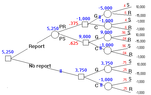
The decision tree:
 Expected value of sample information (EVSI) is the difference between
expected
dollar value with the report which is $5,250 and expected
dollar
value without
the report which is $3,750.
Hence EVSI= $5,250 - $3750 = $1500
Here is another way to arrive at the same results:
If the report predicts Sunny (PS) use probalities of .96 and .04
respectively
for sunny and rainy conditions. In which case the best alternative is
to
go
with the show with EV of $9,000.
Whereas if the report indicates Rainy conditions (PR) use probalities
of .40 and .60 respectively for sunny and rainy conditions. In which
case
the better alternative is to cancel with EV of $-1,000.
There is .625 chance the report will predict sunny in which case we
will go with show and make $9,000 while there is a probability of .375
that the report will predict rain in which case we will cancel and
suffere
a loss of $1,000. Thus the Overall EV:
.625 * 9,000 + .375 * (-1,000) = $5,250 (this is the Expected value
with the report)
Therefore EVSI = EV (with the report) - EV(without the report) = 5,250
- 3,750 = $1,500.
[go to top] [Any
questions?]
 .
.
