 This process of pivoting will continue until all reduced costs
are non-negative at which time an optimal solution will have been
found.
This process of pivoting will continue until all reduced costs
are non-negative at which time an optimal solution will have been
found.In its bare essentials the simplex algorithm is a search method that systematically searches the corners of the feasible solution for an optimal one. It does that by the following procedure:
In the simplex algorithm each BFS is represented by a simplex table that contains information necessary (1)for the testing of the adjacent BFS for improvement; and (2) generating the simplex table that represents the adjacent BFS that offers improvement. Consider the problem:
         MAX  2 X1 +   X2
  SUBJECT TO
         2)   3 X1 + 3 X2 <= 12
         3)     X1 + 3 X2 <=  6
Assume we add slacks SLK 2 and SLK 3 respectively to rows 2 and 3
to convert them into equalities. Thus we have 4 variables and 2
constraints. Remember that at every BFS only two of the four
variables can be non-zero (basic). The simplex table
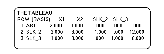
corresponding to the origin (x1=0, x2=0, SLK 2=12, SLK 3=6) is
given:
 The first row is the objective function. The column labeled
(BASIS) always starts with ART, the name of the Objective
function and lists the names of variables that are currently
basic (SLK_2 and SLK_3 here). The first element in the last
column is the current OV, the other entries contain the
corresponding values of these basic variables. Currently OV is
zero SLK_2 is 12 and SLK_3 is 6. (X1 and X2 are zero since they
are not listed under BASIS). The first row under the variable
names contain the "trial" reduced costs (RC). Remember what reduced
cost measures: how much more attractive a variable has
to become before it can be made positive (basic) . Using
this definition we see that a negative RC for a non-basic
(zero) variable indicates that the variable is too attractive not
to be positive. At this point RC of X1 is -2. This signifies that
the OV can be improved by making the value of X1 positive.
However, since we are only interested in BFS, making X1 positive
will require that one of the basic variables, SLK_2 or SLK_3,
become non-basic (zero) to keep the number of positive variables
at two.
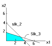
 If you look at
the graph of feasible region you will notice that as X1 increases
the solution (currently at the origin) will slide along the
horizontal axis towards the two constraints and will reach the
first constraint first, making its slack, SLK_2 zero.
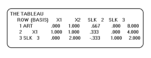
This is a process called PIVOT (a math operation) which takes the
simplex algorithm from one BFS to an adjacent one. The PIVOT that
we described above will introduces X1 into the solution at a
value of 4, making SLK_2 zero (nonbasic). The next BFS therefore
will have X1 and SLK_3 as basic variables and SLK_2 and X2 as
non-basic ones. The simplex table corresponding to this BFS is
given below:
 This process of pivoting will continue until all reduced costs
are non-negative at which time an optimal solution will have been
found.