After the problem is solved and an optimal solution is obtained, a set
of analysis is often conducted to determine the sensitivity of the optimal
solution to changes in problem data, most commonly the objective function
coefficients of variables and the right hand sides of constraints.
These analyses are generally conducted by changing one data element
at a time holding all other data constant.
-
Clearly understand the difference between a problem datum and a problem
variable. In sensitivity, we are allowing one of the problem data to vary,
to see what happens to the optimality of the current solution (a set of
values assigned to decision variables).
-
Example
     Max 5000E + 4000F
     st      E + F       >= 5
             E - 3F      <= 0
           20E + 10F     <= 160
           10E + 15F     <= 150
           30E + 10F     >= 135

[Objective Function] [Right Hand
Sides]
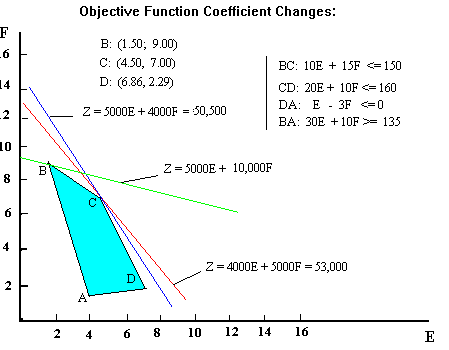
Optimality of point C is preserved for certain changes in the objective
function coefficients of the variables (like in the case of the red contour)
while the optimality shifts to point B, for a more drastic change in the
objective function (as in the case of the green contour).
The critical question of sensitivity analysis is how drastically a coefficient
(data) has to change, before the current solution is no longer optimal
--or before the optimal point shifts to another point.
Sensitivity of the optimal solution (point C) to changes in the coefficient
of F
-
Increases in the coefficient of F.
-
As F becomes more profitable every contour will become flatter since for
any given level of total profit we will now need fewer Fs than before.
If the contours do not become as flat as the line segment BC, point C will
continue being optimal. When, however ,the contour is as flat as line BC,
there will be two optimal corners -- points C and B. Any further increase
in F's coefficient will make the contour too flat to be tangent at C making
point B the unique optimal.
-
We therefore want to calculate the increase in F's coefficient which makes
points C and B optimal at the same time (or equivalently, it makes the
slopes of the contours equal to the slope of line BC).
-
Using the first argument (namely at the allowable maximum of F's coefficient
points B and C are alternative optima) we can calculate this maximum allowable
value. Let ? stand for the coefficient of F.
OV at point C (E=4.5, F=7) equals OV at B (E=1.5, F=9) or
5000*4.5 + ? * 7 = 5000*1.5 + ?*9
solving for "? " we find $7500.
-
So, as long as the coefficient of F does not increase beyond $7500 point
C will remain optimal; at $7500, both point C and point B will be optimal;
and for values more than $7500, point B will be the unique optimal.
-
We can reach the same conclusion by searching for the coefficient of F
that will make the contours as flat as the line segment BC. We can calculate
the slope of a linear line as minus the coefficient of the first variable
(X axis)/the coefficient of the second (Y axis). Thus, we want
slope of a contour = slope of BC
-5000/? = -10/15
solving for ? we obtain $7500 as before.
-
Notice that when F becomes sufficiently profitable the solution shifts
counter-clock wise to take advantage of the more favorable price for F.
At the new optimum more F's are made (9 now) at the expense of E's (only
1.5 now).
-
Decreases in the coefficient of F.
-
As F becomes less profitable, the contours will become steeper. If they
become steep enough, the optimal solution will move in the clock wise direction--
to point D (E= 6.86, F= 2.29). Hence:
5000*6.86 + ?*2.29 = 5000*4.5+?*7
Solving for ? we find $2,500. Also, from the equality of the slopes of
the contours and line CD:
-?/5000 = - 10/20
we find as before the critical value to be $2500.
-
We can conclude that as long as the coefficient of F stays within the interval
from $2500 to $7500, the current optimal values 4.5 for E and 7 for F (point
C) will remain optimal. Notice however, that although the solution is not
changing, the objective function value is changing . In fact, within
this range, the objective function value changes at a rate equal to the
optimal value of the variable whose coefficient is varying. In the
example this is variable F and its optimal value is 7. Thus every dollar
increase in the coefficient of F will produce a $7 increase in the OV as
we are making and selling 7 units of F.
Sensitivity of the Optimal Solution to Changes in the Right Hand Sides
of Constraints

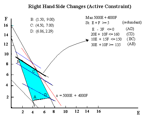
When the right hand side of a constraint changes, the constraint boundary
will move parallel to itself. This will generally change the feasible region
having no effect on the slopes of the objective function contours.
When the RHS of a "<=" type constraint
increases , the constraint
moves in a direction making the feasible region larger. This is called
loosening
the
constraint. Decreases in the RHS of a "<=" constraints will
tighten
the constraint. For a ">=" type constraint the tightening and loosening
directions are reversed.
In the graph if the RHS of 30E + 10F >=135 ( BA) increases, the constraint
moves in the North-East direction shrinking the feasible region, while
if the RHS of 20E + 10F <= 160 (CD) increases, the feasible region will
grow.
-
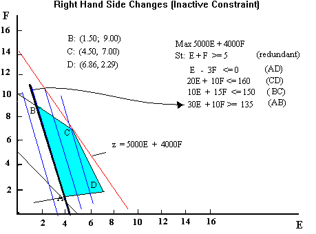
Changing the RHS of an Inactive Constraint .
Consider 30E + 10F >= 135. This is an inactive constraint with a surplus
of 70 units at the point of optimality. If the RHS, decreases line
BA moves away from point C, preserving its optimality; the OV stays the
same; only the surplus of the constraint increases by an amount equal to
the decrease in the RHS.
-
If the RHS increases the constraint moves towards point C. As long as point
C remains on the feasible side of the constraint, its optimality is unaffected;
OV stays the same; only the amount of surplus decreases. When the constraint
shifts sufficiently (by the amount of the surplus) to pass through point
C the constraint becomes active. Any further increase forces the optimal
point to slide down toward point D along line CD.
-
Thus we can conclude that RHS of an inactive constraint can change without
any bound in the loosening direction, and can change by the amount of the
slack/surplus in the tightening direction. In this example the RHS can
vary from minus infinity to 205 without altering the optimality of point
C.
-
Active Constraint

-
Consider 10E + 15F <=150, an active constraint passing through point
C. When the RHS of this constraint decreases, the coordinates of C changes
as it slides down along the line CD towards D. However, point C will remain
optimal (albeit with different E and F values) until point D is reached.
This happens when the RHS is equal to:
10*(6.86) + 15*(2.29) = 102.95.
-
If, on the other hand, the RHS increases the constraint moves up, making
the feasible region larger and moving the point of optimality upwards.
This pattern will continue as long as the constraint remains active. Verify
that the constraint remains active until point (0,16) is reached and that
this happens for a rhs of 240.
-
Thus as the RHS of the constraint changes from 240 to 102.95, point C (the
intersection of CD and BC) stays optimal; the values of the variables change;
the OV changes (increases as the constraint becomes looser, decreases if
as it becomes tighter). This rate at which the OV changes is referred to
as the shadow price of the constraint.
-
The shadow price can be obtained by calculating the OV at the original
optimum point C (4.5, 7). This is is $50,500. And the OV at point D
(6.86, 2.29) -- the optimum solution for a rhs of 102.5. The OV at point
D is $43,460. Thus when the rhs goes down by 150-102.5 = 47.5 units, the
OV goes down by $50,500- $43,460 = $7040. The per unit change in the OV
then is $7,040 / 47.5 = $148.21 (the shadow price). Each unit of decrease
in the rhs of the constraint causes a $148.21 decrease in the OV.
Main Sensitivity Principles
