Error estimates for approximating any Taylor Series

We have talked about estimating the error in approximating the sum of a Taylor series using a Taylor polynomial (or in other words, a partial sum) if the series converges by the Alternating Series Test. However, if the Alternating Series test does not apply, then we need another method for estimating the error. With Maple, we can actually look at the graph of Rn(x) to estimate the error, but this is cheating in the sense that if we can compute the exact error, then that means we can essentially find the exact value of the function and we wouldn't need to be worrying about errors. A more practical and useful method is to use Taylor's Inequality given on page 788 of our text:

> abs(R[n](x))<=M*abs(x-a)^(n+1)/(n+1)!;

The ability to look at essentially exact values of the function under consideration and Rn(x) does enable us to see that Taylor's Inequality does indeed work, and also some sense of how well it works. This can give us intuition into what to expect when we have to deal with a function whose exact values are not so easy to compute.

In the examples, we will use the command taylorfunction from our wfucalc library. If you have installed it on your computer, and are using Maple 6, then give the following command to load the library.

> with(wfucalc);

The taylorfunction command defines a function that is the Taylor polynomial of the expression given as the first parameter, about x = a given as the second parameter, with n+1 terms if n+1 is the third parameter. The polynomial will be of degree n since the constant term is counted as an extra term. For example, if we want the Taylor polynomial of degree 2 for f(x) = sqrt(x) about x = 4 (i.e. when a = 4), then we type:

> T2:=taylorfunction(sqrt(x),x=4,3);

Alternatively, if you don't have the wfucalc library, you can give the following command using only standard Maple procedures.

> T2:=unapply(convert(taylor(sqrt(x),x=4,3),polynom),x);

Note that Maple oversimplifies, since the standard way to write the Taylor polynomial of degree 2 would be T2(x) = 2 + (1/4)*(x-4) - (1/64)*(x-4)^2. Be sure to correct this when you write down your answers; don't let Maple lead you astray. Maple is faster and more accurate than we are, but never smarter.

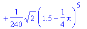
Now, in order to determine the value of M in Taylor's inequality, we need to look at the third derivative of our function. The diff command, given an expression for a function followed by three x's (one for each derivative we want to take), gives us the third derivative of the function.

> d3:=diff(sqrt(x),x,x,x);

Note that the expression x$6 is interpreted by Maple as a list of 6 x's, so that x$3 could be used instead of x,x,x to compute the third derivative.

> x$6;

> d3:=diff(sqrt(x),x$3);

Now if we want to approximate sqrt(x) for x in the interval [4,4.2], then we need the consider the interval symmetric about x = 4, in other words, the interval satisfying |x-4| <= 0.2, or the interval [3.8,4.2] Thus, we graph the absolute value of the third derivative on this interval to see where its maximum value occurs.

> plot(abs(d3),x=3.8..4.2);

Since the maximum occurs at 3.8, we can evaluate the absolute value of the third derivative at 3.8 to define M in Taylor's Inequality. Since d3 has been defined as an expression rather than a function, we use the command eval to evaluate at x = 3.8.

> M:=eval(d3,x=3.8);

The absolute value of the error in using T2 to approximate sqrt(x) on the interval [3.8,4.2] is the value of |R2(x)| that is less than

> M*(0.2)^3/3!;

Thus, we see that the error is less than .00005 so that T2 should give four decimal accuracy for points in the interval [3.8,4.2]. Let us verify this by looking at the values of T2(x) and Maple's ten decimal approximations of sin(x), for x = 4.1, 4.2, and 3.8 remembering that the approximations are generally the worse as we move away from x = 4.

> T2(4.1);

> sqrt(4.1);

> T2(4.2);

> sqrt(4.2);

> T2(3.8);

> sqrt(3.8);

Note that the approximation at x = 4.1 seems to better than the approximations at 3.8 and 4.2. This is no surprise since 4.1 is closer to 4. In fact, we can show that T2(4.1) is good to five decimal places by using x = 4.1 in Taylor's Inequality. |x - 4| = |4.1 - 4| = 0.1. The estimate we used previously works for any x in the interval [3.8,4.2], but for any x in the interval [3.9, 4.1], we can say that the error is less than

> M*(0.1)^3/3!;

Thus T2 gives five decimal accuracy for any x in the interval [3.9,4.1]. We could also compute a smaller M on this interval and get a better estimate, but we do not do so here partly because it does not enable us to conclude greater decimal accuracy at x = 4.1. Next let us compare the above error estimates with the actual error R2(x). We plot abs(R2(x)) to see where it is max and then evaluate it there.

> R2:= x -> sqrt(x)-T2(x);

> plot(abs(R2(x)),x=3.8..4.2);

The maximum error evidently occurs at the endpoints of [3.8,4.2] or of [3.9,4.1].

> abs(R2(3.8));

> abs(R2(4.2));

> abs(R2(3.9));

> abs(R2(4.1));

Our estimate .00001777 compares favorably to the actual maximum error of .000016131 on the interval [3.8,4.2], and our estimate of .000002221 is somewhat larger than the actual maximum of .000001984 on the interval [3.9,4.1]. Finally, we note that if we restrict our attention to the interval [4, 4.2], then the actual maximum error is about .000015153 which is roughly the answer given in the book for problem 13 b on page 807.

Now let us consider approximating sin(x) for x in the interval [0,Pi/2]. Since the midpoint of this interval is Pi/4, and sin(x) and all its derivatives are easily evaluated at x = Pi/4, we will look at a Taylor polynomial for sin(x) about x = Pi/4 (i.e. a = Pi/4). Let us use the Taylor polynomial of degree 5 (6 terms).

> T5:=taylorfunction(sin(x),x=Pi/4,6);

The sixth derivative of sin(x) is either going to be sin(x), cos(x), -sin(x), or -cos(x). In fact, it is

> d6:=diff(sin(x),x$6);

No matter which derivative of sin(x) we wish to bound, we can take M = 1, since |sin(x)| and |cos(x)| never get bigger than 1 on any interval. On some intervals, it may be that M can be taken to be smaller than 1, but on our interval that is not the case and in many cases the extra work to find a smaller M may not be worth the effort. Since M = 1, n = 5, and |x - 4| <= Pi/4, Taylor's Inequality gives us an error bound of

> evalf((Pi/4)^6/6!);

Thus we can expect three decimal accuracy using T5(x) to approximate sin(x) on the interval [0,Pi/2] .

For example

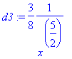
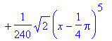
> T5(1.5);

> evalf(%);

> sin(1.5);

1.5 is close to the edge of our interval so it should not be surprising that three decimal accuracy is all that we get. Now lets compare our error estimate to the actual error R5(x).

> R5 := x -> sin(x)-T5(x);

> plot(abs(R5(x)),x=0..Pi/2);

The graph shows that the maximum error occurs at Pi/2. Since we have defined R5 as a function, we can use either eval or R5 itself to find its value at x = Pi/2.

> eval(R5(x),x=Pi/2);

> R5(Pi/2);

> evalf(%);

Note that I did not take absolute values so the value shown is negative. so |R5(x)| <= .000254 ahd also note that the actual error does not guarantee any better than the three decimal accuracy given by Taylor's Inequality.

Now suppose we want to calculate sin(35 degrees). To do this, we must first convert 35 degrees to radians. Recall that halfway around the unit circle is Pi radians = 180 degrees, so 1 degree is Pi/180 radians, thus 35 degrees is

> 35*Pi/180;

Since (7/36) Pi is in our interval [0,Pi/2], we can be assured that we can get three decimal accuracy with the approximation

> T5(7*Pi/36);

> evalf(%);

In fact, since (7/36) Pi is in the interior of our interval, the estimate should be better than the worst case, so we can use Taylor's Inequality to get a better estimate by putting x = (7/36) Pi. Thus, we obtain an error estimate of

> abs(7*Pi/36-Pi/4)^6/6!;

> evalf(%);

Thus our estimate should be good to seven decimal places. Looking at Maple's ten decimal approximation of sin( 7/36 Pi), we see that this is indeed the case.

> evalf(sin(7*Pi/36));