Jan 29, 2001
Notes for Lecture
Notes for Lecture #5
Methods for solving Poisson equation
There are are large number of tools for solving the Poisson and
Laplace equations:
- Green's function methods:
|
F(r) = |
1
4pe0
|
|
ó
ő
|
V
|
d3r˘ r(r˘) G(r,r˘) + |
1
4p
|
|
ó
ő
|
S
|
|
é
ę
ë
|
G(r,r˘) |
¶F
¶n˘
|
- F(r˘) |
¶ G(r,r˘)
¶n˘
|
ů
ú
ű
|
da˘. |
| (1) |
- Complete function expansions; Fourier series, etc.
- Variational methods
- Grid based methods
Introduction to grid-based methods
The basis for most grid-based methods is the Taylor's expansion:
|
F(r + u ) = F(r) + u·Ń F(r) + |
1
2!
|
(u·Ń)2 F(r) + |
1
3!
|
(u·Ń)3 F(r) + |
1
4!
|
(u·Ń)4 F(r) + Ľ. |
| (2) |
We will work out some explicit formulae for a 2-dimensional
regular grid with h denoting the step length. For the
2-dimensional Poisson equation we have
|
|
ć
ç
č
|
|
¶2
¶x2
|
+ |
¶2
¶y2
|
ö
÷
ř
|
F(x,y) = - |
r(x,y)
e0
|
. |
| (3) |
We note that a sum of 4 surrounding edge values gives:
|
| |
|
|
|
F(x+h,y) + F(x-h,y) + F(x,y+h) + F(x,y-h) |
| (4) | |
|
| 4F(x,y) + h2 |
ć
ç
č
|
¶2
¶x2
|
+ |
¶2
¶y2
|
ö
÷
ř
|
F(x,y) + |
h4
12
|
|
ć
ç
č
|
|
¶4
¶x4
|
+ |
¶4
¶y4
|
ö
÷
ř
|
F(x,y) + (h6Ľ). |
|
| |
|
Similarly, a sum of 4 surrounding corner values gives:
|
| |
|
|
|
F(x+h,y+h) + F(x-h,y+h) + F(x+h,y-h) +F(x-h,y-h) |
| (5) | |
|
| 4F(x,y) + 2h2 |
ć
ç
č
|
¶2
¶x2
|
+ |
¶2
¶y2
|
ö
÷
ř
|
F(x,y) + |
h4
6
|
|
ć
ç
č
|
|
¶4
¶x4
|
+ |
¶4
¶y4
|
+ 6 |
¶2
¶x2
|
|
¶2
¶y2
|
ö
÷
ř
|
F(x,y) +(h6Ľ). |
|
| |
|
We note that we can combine these two results into the relation
|
SA + |
1
4
|
SB = 5 F(x,y) + |
3h2
2
|
Ń2F(x,y)+ |
h4
8
|
Ń2 Ń2 F(x,y) + (h6Ľ). |
| (6) |
This result can be written in the form;
|
F(x,y) - |
1
5
|
SA - |
1
20
|
SB = |
3h2
10 e0
|
r(x,y) + |
h4
40 e0
|
Ń2 r(x,y). |
| (7) |
In general, the right hand side of this equation is known, and
most of the left hand side of the equation, except for the
boundary values are unknown. It can be used to develop a set of
linear equations for the values of F(x,y) on the grid points.
For example, consider a solution to the Laplace equation in the
square region 0 Ł x Ł a, 0 Ł y Ł a which
F(x,0) = F(0,y) = F(a,y) = 0 and F(x,a) = V0. We will
first analyze this system with a mesh of 9 points. In this case,
f5 ş F(a/2,a/2) is unknown, while
f1 = f2 = f3 = 1 and
f4 = f6 = f7 = f8 = f9 = 0.
Figure
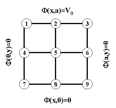 For this example, Eq. 7 states
|
f5 = |
1
5
|
(f2+f4+f6+f8)+ |
1
20
|
(f1+f3+f7+f9) = |
3
10
|
V0. |
| (8) |
This results is within 20% of the exact answer of
F(a/2,a/2) = 0.25 V0. If analyze this same
system with the next more accurate grid, using the symmetry of the
system F(x,y) = F(a-x,y), we have now 6 unknown values
{f5,f6,f8,f9,f11, f12} and
boundary values f1 = f2 = f3 = 1 and
f4 = f7 = f10 = f13 = f14 = f15 = 0.
Figure
 This results in the following relations between the grid points:
|
f5- |
1
5
|
(f2+f4+f6+f8) - |
1
20
|
(f1+f3+f7+f9) = 0, |
| (9) |
|
f6- |
1
5
|
(f3+f5+f5+f9) - |
1
20
|
(f2+f2+f8+f8) = 0, |
| (10) |
|
f8- |
1
5
|
(f5+f7f9+f11) - |
1
20
|
(f4+f6+f10+f12) = 0, |
| (11) |
|
f9- |
1
5
|
(f6+f8+f8+f12) - |
1
20
|
(f5+f5+f11+f11) = 0, |
| (12) |
|
f11- |
1
5
|
(f8+f10+f12+f14) - |
1
20
|
(f7+f9+f13+f15) = 0, |
| (13) |
|
f12- |
1
5
|
(f9+f11+f11+f15) - |
1
20
|
(f8+f8+f14+f14) = 0. |
| (14) |
These equations can be cast into the form of a matrix problem
which can be easily solved using Maple:
| | | | | |
| |
| | | | | |
| |
| | | | |
|
) |
|
|
| |
|
| |
|
| |
|
| |
|
|
) = |
|
|
| |
|
| |
|
| |
|
| |
|
|
) V0. |
(15) |