
With Kaitlin Hill and Xuan Kelsy Fei, I studied noise-induced transitions from a perennially ice-covered Arctic state to an ice-free state in the periodically forced energy-balance model introduced by Eisenman and Wettlaufer. The central question is a rare-event problem: when both the ice-covered and ice-free seasonal states are deterministically stable, what path is a stochastically forced system most likely to follow when it transitions from one climate state to the other? The problem is mathematically interesting because the competing climate states are periodic orbits rather than equilibria and because the thermodynamics change when sea ice disappears, producing a piecewise-smooth dynamical system.
Arctic energy-balance model
The state variable \(E(t)\) is the vertically integrated energy per unit surface area of the Arctic column. Negative values of \(E\) correspond to sea ice, with energy related to ice thickness, while positive values correspond to an ice-free ocean mixed layer, with energy related to ocean temperature. We introduce stochastic forcing through
\[ dE_t=f(t,E_t)\,dt+\sigma\,dW_t. \]The drift \(f(t,E)\) is periodically forced by the annual radiation cycle and changes form according to the physical state of the Arctic. A compact representation is
\[ f(t,E)= \begin{cases} p_{ml}(t)-\dfrac{F_T(t)}{c_{ml}H_{ml}}E+F_B, & E>0,\\[6pt] p_i(t)+F_B-\nu_0E, & E<0,\quad p_i(t)>0,\\[6pt] p_i(t)-\dfrac{p_i(t)F_T(t)E}{F_T(t)E-k_iL_i}+F_B-\nu_0E, & E<0,\quad p_i(t)\le 0. \end{cases} \]Thus \(E=0\) is more than a mathematical boundary: it separates two different physical regimes. On the ice-covered side, the model describes the growth and melting of sea ice; on the positive-energy side, it describes heating and cooling of an exposed ocean mixed layer. This switching structure is what makes the drift piecewise smooth.
Bistability and noise-induced tipping
Because the forcing is annual, the relevant deterministic climate states are periodic solutions. In the bistable parameter regime, one attracting annual cycle represents a perennially ice-covered Arctic and another represents a perennially ice-free Arctic. A noise-induced transition is therefore not a jump between two equilibria. Instead, a trajectory must leave the neighborhood of one attracting seasonal cycle, pass through the ice-loss boundary \(E=0\), and approach the other attracting cycle.
This distinction is important for understanding the timing of a transition. The stability of the ice-covered state and its distance from the switching boundary vary throughout the seasonal cycle. Consequently, the likelihood of escape depends not only on the amount of noise but also on the time of year at which a rare fluctuation begins to move the system away from its attracting cycle.
Most probable transition path
For small noise, Freidlin-Wentzell large-deviation theory associates a cost with each candidate transition path. Because the original drift is piecewise smooth, we work with a smooth approximation \(f_\varepsilon\) and minimize the action
\[ I_\varepsilon[\phi] = \frac12\int_{t_0}^{t_f} \left(\dot\phi-f_\varepsilon(t,\phi)\right)^2\,dt. \]The minimizer identifies the path requiring the least unlikely realization of the stochastic forcing and hence gives the most probable route for a rare transition in the small-noise limit. We compute this path numerically by evolving a gradient flow for the action functional. This converts the rare-event problem into a variational calculation rather than requiring us to wait for extremely uncommon transitions to appear in direct simulation.
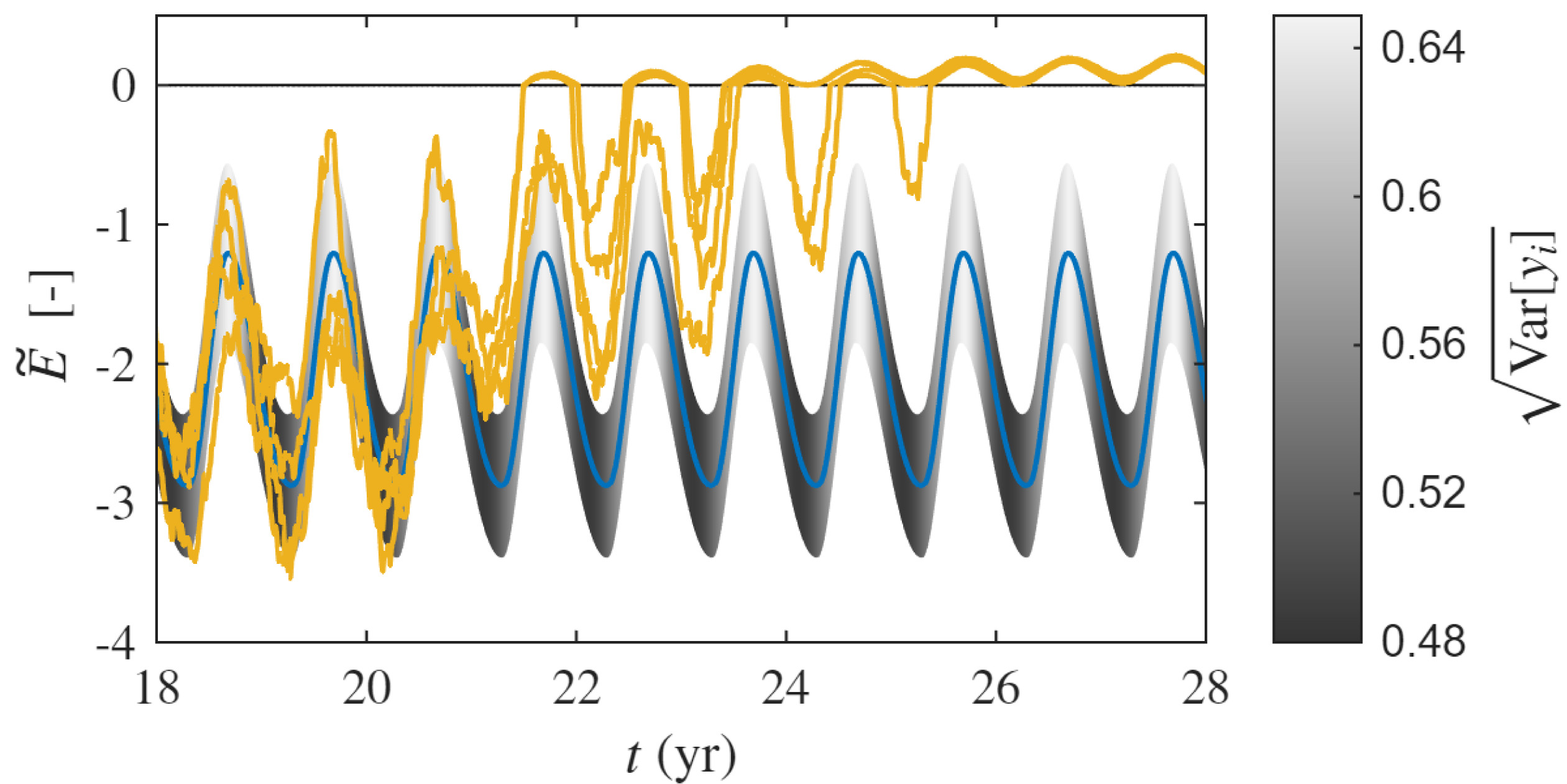
We then compare the calculated minimizer with ensembles of Monte Carlo simulations. The transition trajectories shown in the figure move from the lower, ice-covered seasonal cycle toward the upper, ice-free cycle. Successful stochastic transitions concentrate around the predicted transition route. They also exhibit a pronounced seasonal dependence: transitions typically begin during the first half of the year and develop over many annual cycles rather than occurring as an instantaneous loss of sea ice.
Estimating transition times
The most probable path describes how a rare transition occurs, but a second question is how long one should expect to wait for such an event. Near a stable periodic orbit \(E_s(t)\), we write
\[ E(t)=E_s(t)+Y(t) \]and linearize the stochastic dynamics. The perturbation \(Y(t)\) then satisfies a periodically forced Ornstein-Uhlenbeck-type equation,
\[ dY=a(t)Y\,dt+\sigma\,dW_t. \]This approximation can be used to construct an effective quasi-potential measuring the stochastic barrier between the attracting periodic orbit and the switching manifold. The barrier determines the exponential scale of the mean escape time, playing a role analogous to the potential barrier in Kramers' law while accounting for the periodically varying stability of the Arctic climate state.
Why the piecewise-smooth structure matters
Any transition from a perennially ice-covered state to an ice-free state must cross \(E=0\), precisely where the physical interpretation of the state variable and the governing thermodynamic law change. The transition therefore probes the nonsmooth part of the model rather than remaining within a single smooth regime. This makes the Arctic energy-balance model a natural application of our work on rare transitions in piecewise-smooth stochastic dynamical systems: the mathematical difficulty created by the switching boundary is directly connected to the physical process of losing sea ice.
Reference
- Hill, K., Fei, X. K., & Gemmer, J. A. (2026). Most probable transition path to an ice-free state in a model for Arctic energy balance. Chaos 36, 093113.