
With Gary Moon and Sarah Raynor, I studied a two-dimensional, two-phase elliptic free-boundary problem with Neumann boundary conditions. The basic difficulty is that the interface separating the positive and negative phases is not prescribed in advance. Instead, both the function and the location of the interface must be determined as part of the variational problem. A motivating example is the steady flow of two immiscible, incompressible fluids: the velocity potential is harmonic in each fluid, while a jump condition must hold where the two fluids meet.
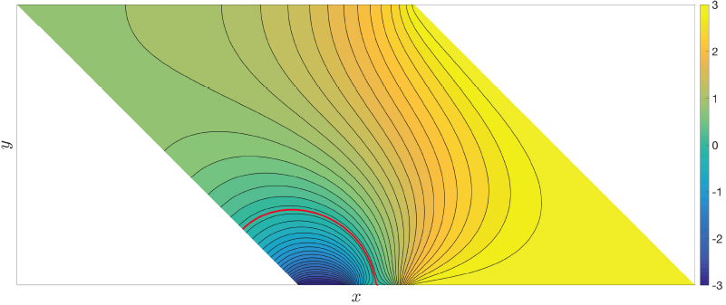
The figure above shows a numerical solution of the free-boundary problem on a polygonal domain. The colored field represents the computed solution \(u\), while the interface separating the positive and negative phases is the free boundary. The calculation illustrates the central geometric issue in this project: how an interface that is determined by the variational problem approaches and interacts with the fixed Neumann boundary, particularly near a corner where the direction of that boundary changes abruptly.
Variational formulation
Let \(\Omega\subset\mathbb R^2\) be a bounded convex domain and write its fixed boundary as the union of a Dirichlet portion \(S\) and a Neumann portion \(N\). We study local minimizers of
\[ J[v]=\int_\Omega\left(|\nabla v|^2+Q^2(x)\lambda^2(v)\right)\,dx, \]where \(Q\) is bounded above and below by positive constants and
\[ \lambda(v)= \begin{cases} \lambda_1, & v>0,\\ \lambda_2, & v\le 0, \end{cases} \qquad \lambda_1>\lambda_2>0. \]The admissible functions satisfy prescribed data on \(S\), while the Neumann condition on \(N\) arises naturally from the variational principle. If \(u\) is a minimizer, then it is harmonic in each phase,
\[ \Delta u=0\qquad\text{in }\{u>0\}\cup\{u<0\}, \]satisfies the Neumann condition \(\partial_\nu u=0\) weakly on \(N\), and has free boundary
\[ \Gamma=\partial\{u>0\}\cap\Omega. \]Along \(\Gamma\), the two phases are coupled by the Bernoulli-type jump condition
\[ |\nabla u^+|^2-|\nabla u^-|^2 =(\lambda_1^2-\lambda_2^2)Q^2(x). \]The location of \(\Gamma\) is therefore determined by a balance between the Dirichlet energy and the energetic cost assigned to the two phases. This is what makes the problem a free-boundary problem rather than an elliptic equation on a predetermined domain.
Regularity at a Neumann boundary
A central analytical question is whether the regularity known for two-phase minimizers in the interior persists all the way to a nonsmooth fixed boundary. We prove that, in two dimensions, minimizers are Lipschitz continuous up to a convex Neumann boundary away from the Dirichlet portion. Convexity is important: near a re-entrant corner even an ordinary harmonic function can fail to be Lipschitz.
The proof adapts the Alt–Caffarelli–Friedman monotonicity method to the boundary. Near a point of the Neumann boundary we control a scale-dependent product of the Dirichlet energies of the positive and negative phases. Convexity bounds the angular geometry of those phases and allows the corresponding monotonicity formula to survive at the boundary. Combined with estimates on the measure \(\Delta u\), harmonic comparison functions, and boundary Harnack-type estimates, this yields a uniform gradient bound for the minimizer.
Why corners create a geometric obstruction
Away from a corner, a smooth free boundary meeting a Neumann boundary is expected to intersect it orthogonally. At a polygonal corner, however, this local orthogonality requirement competes with the global continuity of the free boundary. For an obtuse corner there is enough room for the terminal point of the free boundary to move continuously from one side of the corner to the other. At an acute corner, orthogonality prevents the free boundary from approaching the vertex arbitrarily closely. The computations consequently reveal a neighborhood of the corner that is not visited by steady free boundaries, producing a numerical ``forbidden region.''
Numerical approximation
Directly minimizing \(J\) is difficult because the phase term is discontinuous at \(u=0\). We therefore replace it by a smooth transition layer \(\phi_\varepsilon(u)\), producing the relaxed functional
\[ J_\varepsilon[v] = \int_\Omega\left(|\nabla v|^2+Q^2(x)\phi_\varepsilon(v)\right)\,dx. \]The regularized minimizers satisfy a nonlinear Poisson equation, and we compute them by evolving the gradient flow
\[ v_t=2\Delta v-Q^2(x)\phi_\varepsilon'(v). \]The energy \(J_\varepsilon\) is a Lyapunov function for this evolution, so the flow decreases the relaxed energy and approaches a local minimizer. The free boundary does not have to be tracked explicitly: after convergence it is recovered simply as the zero contour of \(v\). This is especially useful when the topology of the zero set changes during the evolution.
Finite-difference scheme on parallelograms
For the numerical experiments, polygonal geometry is represented by parallelograms parameterized by an opening angle \(\theta\). Mapping the parallelogram to a unit square introduces a mixed derivative into the Laplacian. We discretize the resulting equation on a uniform grid using second-order centered finite differences. Ghost points enforce the Neumann conditions along the two Neumann sides, and the time evolution is computed with the Crank–Nicolson method.
The transition-layer width is tied to the spatial mesh by setting \(\varepsilon=2h\). Thus the regularization becomes sharper as the grid is refined. Convergence is assessed by monitoring \(J_\varepsilon\) along the gradient flow and then refining the mesh until the steady-state energy stabilizes. This choice is also connected to the analysis: minimizers of the relaxed energies converge, along subsequences, in \(H^1\) to minimizers of the original free-boundary functional.
What the computations show
The boundary data contain an amplitude parameter \(A\) that acts as a control parameter for the terminal position of the free boundary. Increasing \(A\) pushes the interface toward and eventually past the Neumann corner. For an obtuse angle, the terminal point moves smoothly through the corner. For a right angle, the numerical solution appears to jump from one Neumann side to the other, although the distance of closest approach scales with the mesh size, making it difficult to separate genuine behavior from discretization effects.
The acute-angle case is qualitatively different. Under mesh refinement the jump persists, and the steady free boundary never enters a neighborhood of the corner. During the gradient flow the interface can temporarily split, creating a transient zero phase around the vertex before settling onto the other Neumann boundary. The slow evolution immediately before the jump and rapid motion afterward are suggestive of a loss of a local minimum of the relaxed energy. These computations therefore point to a richer variational structure near acute corners, potentially involving multiple local minimizers as well as a geometrically enforced forbidden region.
Reference
- Gemmer, J. A., Moon, G., & Raynor, S. G. (2020). Solutions to a two-dimensional, Neumann free boundary problem. Applicable Analysis 99(2), 214–231.