
My work on retinal coding with Shai Sabbah and collaborators asks how a curved sensory surface represents geometric information in the visual world. Two related projects address this question from complementary directions. Our 2017 Nature paper studied direction-selective ganglion cells (DSGCs) and showed that their preferred directions are organized by global optic-flow geometry. Our 2025 Cell Reports paper studied orientation-selective ganglion cells (OSGCs) and found a related spherical organization for the representation of edges. In both cases, patterns that appear complicated on a flattened retina become much more organized when the geometry of the intact eye is taken into account.
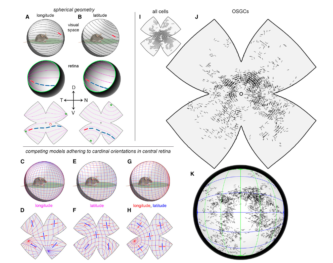
The image above illustrates this basic geometric viewpoint for orientation-selective cells. Local preferred orientations vary across the retina, but those local measurements can be interpreted as samples of simple orientation fields defined on the curved retinal surface. The same geometric issue arose in our earlier work on direction selectivity: measurements are made on a retina that has been cut and flattened for imaging, whereas the visual motion being represented is naturally defined on the approximately hemispherical retina of the intact eye.
Why retinal geometry matters
Consider a point on the retina represented by a unit vector \(r\in S^2\), and let \(a\in S^2\) denote an axis in visual space. Translation along the axis \(a\) generates a tangent direction obtained by projecting \(a\) onto the tangent plane of the sphere:
\[ \tau_{\mathrm{trans}}(r;a) = \frac{a-(a\cdot r)r} {\|a-(a\cdot r)r\|}. \]By contrast, rotation about the axis \(a\) produces a tangent direction proportional to
\[ \tau_{\mathrm{rot}}(r;a) = \frac{a\times r}{\|a\times r\|}. \]Thus a single global motion does not correspond to a constant direction across the retina. Its local direction changes systematically with position. This is the central geometric idea behind the 2017 study: if a population of DSGCs represents a particular global optic-flow field, then the preferred direction of individual cells should vary across the retinal surface in exactly the way prescribed by that field.
Direction selectivity and the retinal code for self-motion
In the 2017 Nature study, we measured the preferred directions of more than 2,400 DSGCs at known locations across 26 mouse retinas. The preferred directions were not globally fixed at the four cardinal retinal directions. Instead, they rotated systematically with retinal location. Once the data were reconstructed on the curved retina, each DSGC subtype closely followed the optic flow generated by translation along a particular axis in space.
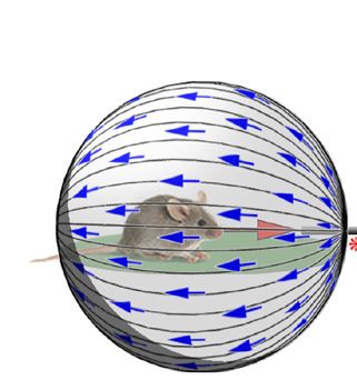
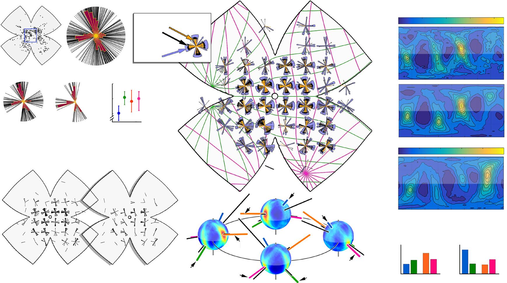
The images above show the connection between local direction preferences and global optic flow. The left image illustrates how translation through space produces a position-dependent motion field on the retina. The right image shows how measured DSGC preferences can be compared with these spherical flow fields. The four ON-OFF DSGC subtypes form four panoramic channels associated with forward and backward translation along the body axis and upward and downward translation along an axis closely aligned with gravity. ON DSGCs unexpectedly follow essentially the same global geometry.
Reconstructing the curved retina from a flat mount
A substantial mathematical problem was therefore to recover the geometry of the intact retina from the flat-mounted tissue used in the experiments. The flattening cannot be treated as a simple projection because cutting and pressing a curved elastic surface into the plane introduces nonuniform stretching and changes both cell positions and preferred-direction vectors.
We modeled the intact retina as part of a sphere of radius \(R\). A point on this spherical retina was described by intrinsic coordinates \((s,\theta)\), where \(s\) is arc length measured from the optic disc and \(\theta\) is the longitudinal angle. The corresponding point in three-dimensional space is
\[ x(s,\theta) = \left( R\sin\!\left(\frac{s}{R}\right)\cos\theta,\, R\sin\!\left(\frac{s}{R}\right)\sin\theta,\, R-R\cos\!\left(\frac{s}{R}\right) \right). \]Here \(x\) is the map from intrinsic retinal coordinates to the spherical retina. The experimental retina contained four relieving cuts used to flatten the tissue. These cuts divide the coordinate domain into four sectors, denoted by \(\Omega_i\). On each sector, the map from the spherical coordinates \((s,\theta)\) to planar coordinates \((u,v)\) on the flat-mounted retina was written as
\[ F(s,\theta)=(u(s,\theta),v(s,\theta)) = \left( \rho_i(s,\theta)\cos f_i(s,\theta),\, \rho_i(s,\theta)\sin f_i(s,\theta) \right). \]The functions \(\rho_i\) and \(f_i\) describe, respectively, the radial and angular coordinates of a material point after flattening. They are not prescribed in advance. Instead, the flattening map \(F\) is determined by treating the retina as an isotropic, incompressible elastic material and minimizing the in-plane elastic energy
\[ E[F] = \sum_{i=1}^{4} \int_{\Omega_i} \left[ \nu(\gamma_{11}+\gamma_{22})^2 + (1-\nu) \left( \gamma_{11}^2+2\gamma_{12}^2+\gamma_{22}^2 \right) \right] \sin\!\left(\frac{s}{R}\right)\,ds\,d\theta . \]In this expression, \(\nu=1/2\) is the Poisson ratio associated with the incompressibility assumption, and \(\gamma_{11}\), \(\gamma_{12}\), and \(\gamma_{22}\) are the components of the in-plane strain tensor generated by the flattening map. The four sectorwise maps are coupled by continuity conditions along the relieving cuts. The experimentally observed flat mount is therefore modeled as the minimum-strain deformation of the spherical retina that is consistent with the measured cut locations and retinal dimensions.
Numerical reconstruction
The variational problem was solved numerically. Each of the four sectors was discretized on a \(40\times40\) uniform grid in \((s,\theta)\). The elastic-energy integral was approximated by composite quadrature, and the derivatives appearing in the strain tensor were approximated with fourth-order finite differences, using one-sided formulas near the sector boundaries. After imposing the continuity conditions along the cuts, the resulting discrete nonlinear least-squares problem was minimized in MATLAB using lsqnonlin.
The numerical minimizer gives a mesh of planar points
\[ (u_{ij},v_{ij})=F(s_{ij},\theta_{ij}), \]which approximates the experimentally observed flat-mounted retina. An experimentally measured cell at planar coordinates \((u,v)\) can then be associated with intrinsic coordinates \((s,\theta)\) through a numerical approximation of \(F^{-1}\). Composing this inverse with the spherical map \(x\) gives
\[ x\circ F^{-1}, \]which reconstructs the cell's location on the three-dimensional retina. To pool data from different animals, we also constructed a standardized flat retina with its own flattening map \(F'\). The composition \(F'\circ F^{-1}\) maps each experimentally measured retina into this common coordinate system.
The reconstruction must also correct preferred directions, not just cell locations. A direction measured on the flat mount is a tangent vector, and flattening can rotate and shear that vector. If \(W\) denotes the measured direction vector in the planar \((u,v)\) coordinates and
\[ J= \begin{pmatrix} \partial u/\partial s & \partial u/\partial\theta\\ \partial v/\partial s & \partial v/\partial\theta \end{pmatrix} \]is the Jacobian matrix of the flattening map, then \(J^{-1}W\) gives the corresponding vector in the intrinsic \((s,\theta)\) coordinates. From there, the vector can be mapped either onto the reconstructed spherical retina or onto the standardized flat retina. This step is essential because the biological comparison concerns the angle between the measured preferred direction and the predicted optic-flow direction, and that angle must be computed after accounting for the geometric distortion introduced by flattening.
Comparing retinal data with optic flow
With cell positions and preferred directions expressed in a common geometric coordinate system, we could compare the data directly with candidate optic-flow fields. For each possible axis of translation, we computed the local optic-flow direction at every measured cell and compared it with that cell's preferred direction. The concordance index was defined as the percentage of cells whose preferred directions differed by less than \(10^\circ\) from the predicted local flow. Repeating this calculation over 2,701 possible translation axes produced a spherical flow-tuning map whose maxima identify the translations best aligned with a DSGC population.
This analysis revealed two pairs of approximately opposing DSGC channels. The N- and T-cell populations encode opposite translations along an axis close to the animal's body axis, while the D- and V-cell populations encode opposite translations along an axis close to gravity. The important point is that this global organization is not apparent from a collection of local preferred directions alone. It emerges after the measurements are interpreted using the geometry of the curved retina.
From direction selectivity to orientation selectivity
Our 2025 work asks a closely related question for edge orientation rather than motion direction. Orientation differs mathematically from direction because an unoriented line has no arrow: the angles \(\theta\) and \(\theta+\pi\) represent the same orientation. A convenient representation is therefore the doubled-angle vector
\[ q(\theta)=(\cos 2\theta,\sin 2\theta), \]which automatically identifies angles that differ by \(\pi\). As in the DSGC problem, the key question is whether locally measured preferences across the retina are samples of a simpler global field on the sphere.
Four OSGC types and a non-orthogonal spherical code
More than 2,100 orientation-selective cells were identified and clustered into four functional types: TON-OFF, SON-OFF, TON, and SON. Their preferred orientations appear approximately horizontal or vertical near the central retina, but rotate systematically with retinal position. Three of the four types are well described by longitude-like orientation fields and one by a latitude-like field.
A particularly interesting feature is that the preferred global fields are not exactly orthogonal. For example, the two dominant TON-OFF longitudinal fields are separated by about \(100^\circ\), or equivalently \(80^\circ\) when interpreted as unoriented axes. A geometric decoder shows that this departure from orthogonality can improve the decoding of edge orientation once spherical projection and biological noise are taken into account.
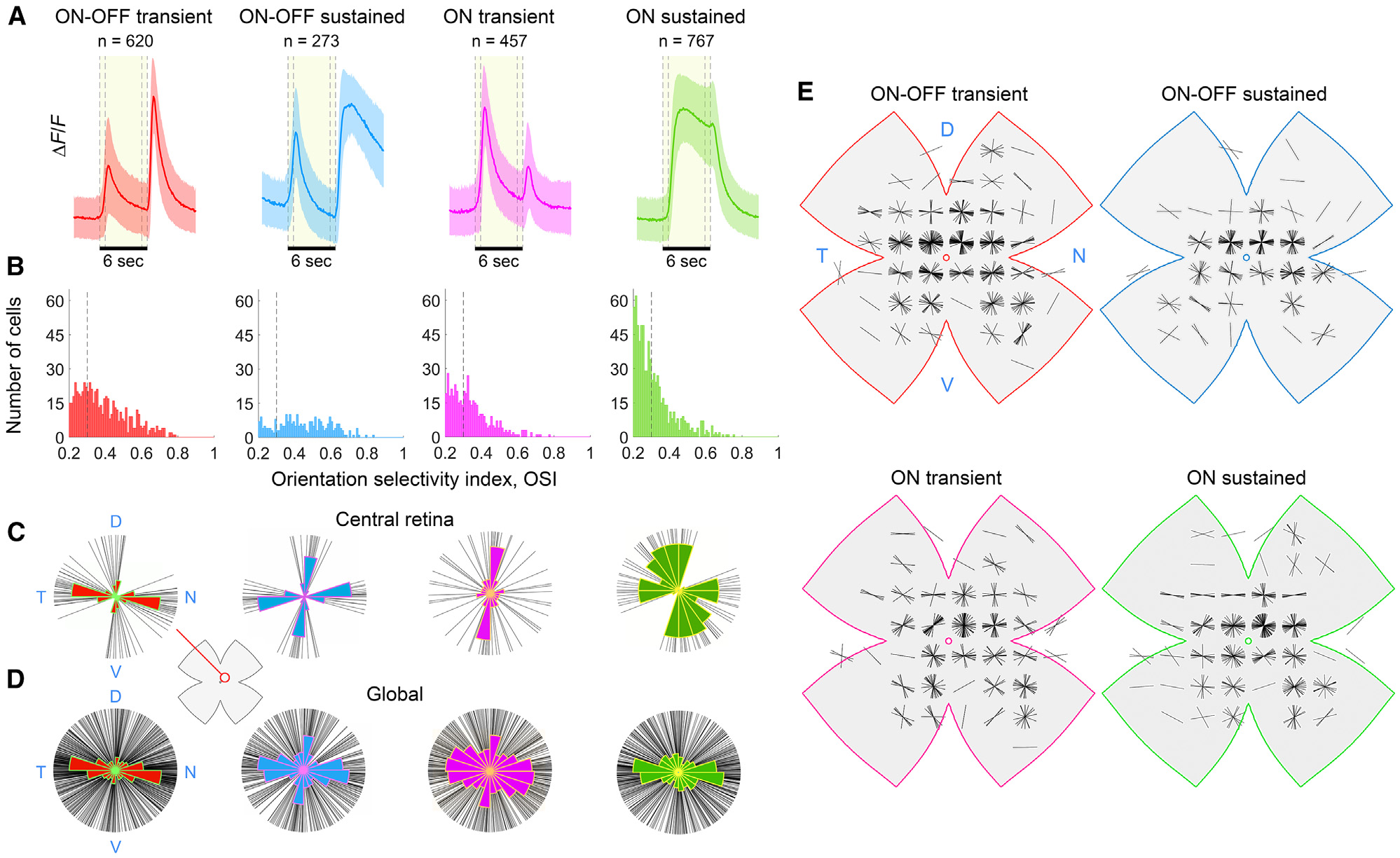
The image above shows the four OSGC response classes and their topographic organization. As with the direction-selective cells, the changing local preferences are not random variations. They reflect a coherent geometric organization across the curved retinal surface.
A common geometric principle
Taken together, the two projects point to a common principle. Direction and orientation preferences that appear spatially variable on a flat-mounted retina can represent simple global structures when viewed on the sphere. For DSGCs, this organization produces channels tuned to optic flow and self-motion. For OSGCs, it produces spherical orientation fields that support the decoding of edge orientation. In both cases, the mathematics provides the link between local measurements made on a flattened biological tissue and the global visual geometry represented by the intact eye.
References
- Sabbah, S., Gemmer, J. A., Bhatia-Lin, A., Manoff, G., Castro, G., Siegel, J. K., Jeffery, N., & Berson, D. M. (2017). A retinal code for motion along the gravitational and body axes. Nature 546, 492–497. doi:10.1038/nature22818.
- Laniado, D. D., Maron, Y., Gemmer, J. A., & Sabbah, S. (2025). A spherical code of retinal orientation selectivity enables decoding in ensembled and retinotopic operation. Cell Reports 44, 115373. doi:10.1016/j.celrep.2025.115373.