Noise Induced Tipping
In the 70's Hasselman introduced a simple climate model consisting of a differential equation perturbed by weak noise:
\[ dx_t=f(x_t,t)dt+\sigma dW,
\]
where the state of the system \(x_t\in \mathbb{R}\) is a stochastic process parametrized by time \(t\geq 0\), \(\,\,f:\mathbb{R}\times [0,\infty)\mapsto \mathbb{R}\) is the drift, \(0< \sigma \ll 1\), and \(W\) is a standard Wiener process. In this equation \(f\) is a proxy for predictable effects that drive the climate on long time scales (years, decades, centuries, millennium), i.e. solar radiation, Earth's albedo, slow changes in orbital parameters etc. The weak noise perturbation models the averaged effects over the many degrees of freedom that occur on short time scales (days), i.e. the weather. While generically we might expect that typical solution trajectories to this equation will essentially track the deterministic dynamics, i.e. solution trajectories for \(\sigma=0\), the presence of noise can have drastic effects on the realized dynamics of the system. Indeed, on long time scales and for time independent drift, the system can undergo "large deviations" away from the deterministic flow leading to rare events such as trajectories crossing over from one (deterministic) domain of attraction to another at the so called Kramer's rate. For time dependent drift, however, the analysis of this equation is more nuanced. Indeed, for time periodic forcing in addition to standard rare events the system can undergo "stochastic resonance" in which solution trajectories periodically transition between stable periodic orbits on time scales on the order of the period of the forcing. In climate models, such transitions between metastable states have been coined "tipping events" and much current research has been focused on determining the parameter regimes in which the crossover between metastable states is likely to occur on relatively short time scales (decades, centuries).
One model for the time evolution for the level of sea-ice in the Arctic Ocean that falls within this framework was proposed by Eisenmann and Weitloffer: \[ \frac{dE}{dt}=(1-\alpha(E))F_s(T)-F_l(t)-T(t,E)+\Delta F_0, \] where \(E\) denotes the latent heat or sensible heat when \(E < 0\) or \(E>0\) respectively, \(\alpha\) is the energy dependent albedo, i.e reflectivity, of the ocean, \(F_s\) denotes seasonally varying incident short wave radiation, \(F_{l}\) denotes (observed) time varying outgoing long wave radiation accounting for seasonal variations in the arctic atmosphere, \(\Delta F_0\) is a perturbation of the surface heat flux, and \(T\) models the surface temperature of the ocean. In this model the ice-covered or ice-free states correspond to \(E<0\) or \(E>0\) respectively and \(\alpha\), \(T\) are piecewise defined to account for phase dependent parameters. It was shown by eisenmann and Weitloffer that for physically realistic definitions of \(\alpha\) and \(T\) the stable periodic orbits for this system undergo saddle-node bifurcations as \(\Delta F_0\) is varied. Specifically, changes in the surface temperature can cause the system to "tip over" from having perennially ice-covered states to having either seasonally ice-covered states or perennially ice free states.
Our Work:
In collaboration with Mary Silber, Yuxin Chen and Alexandria Volkening I am studying noise induced tipping events in periodically driven systems perturbed by additive noise. While our work was initially motivated by the Eisenmann and Weitloffer model we have instead switched our focus to the "toy" system: \[ dx_t=\epsilon^{-1}\left( x-x^3+Bx^2+C+A\cos(t)\right)dt+\sigma dW, \] where \(A,B,C\) are parameters, \(\epsilon\) is the ratio of the rate of relaxation to deterministic steady states to the driving frequency and $\sigma$ is the noise intensity. For various asymptotic regimes, different and interesting behaviors can be observed:
Through Plancherel's indentity it can be shown that the GS algorithm is an error reducing algorithm in the sense that \(I[\varphi_{n+1}]\leq I[\varphi_n]\). However, this property alone does not guarantee convergence of the algorithm. In particular, while projection algorithms converge when the projections are onto convex sets, for fixed \(s\) or \(\Omega\) the projections employed by the GS algorithm are equivalent to projections onto the boundary of the unit ball in \(\mathbb{C}\) which is clearly not convex. This lack of convexity commonly leads to stagnation of the algorithm away from the global minimum which must be overcome by additional ad hoc means. However, while in phase retrieval it is clear that the minimum value is zero, for the optimization problem we considered this is not the case and in fact the minimum may be significantly bounded away from zero. Therefore, when applied to this variational problem it is not clear a priori what a sufficient convergence criterion for the GS algorithm would be.
Method of stationary phase:
We developed an adapted version of the GS algorithm to avoid this stagnation issue. Namely, we used the method of stationary to construct a phase \(\phi\) that satisfies \(\lim_{k\rightarrow \infty} I[\phi]=0\). The phase is constructed as follows:
Uncertainty principle:
Moreover, using essentially the uncertainty principle we proved ansatz free lower bounds on the minimum value of this functional which quantify that a necessary condition for accurate beam shaping is that \[ \beta=\frac{2kW_TW_0r_0}{4z_d^2-W_T^2}>\pi. \] The central result of our work is the identification of the dimensionless quantity \(\beta\)'s critical role in determining the accuracy and applicability of phase shaping in term of the design parameters. Namely, we identified three scaling regimes:
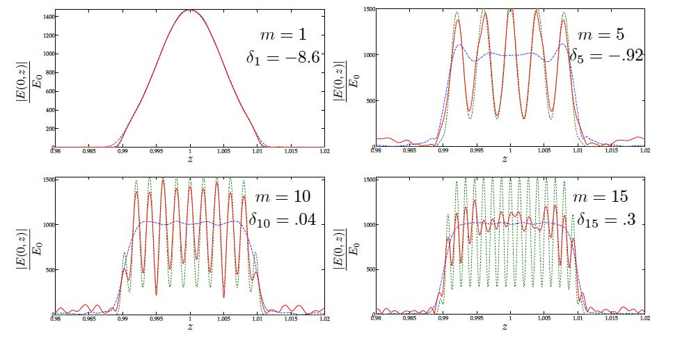
The figure below illustrates our theory in practice. The dashed green curve is the target profile, blue the intensity profile generated by the stationary phase ansatz, red the result of using the GS algorithm with our stationary phase ansatz as the initial guess. The value \(\delta\) is a local measure of \(\beta\) and for positive values our theory predicts that phase shaping will do a poor job of matching the target intensity. In particular, phase shaping is unable to resolve the small scale features in the target intensity profile.
Outlook:
Our work has primarly been concerened with phase shaping the linear optical regime. For more realistic implementations it is necessary to consider the role that turbulence plays in the phase shaping and how additional techniques such as adaptive optics can be deployed to compensate for atmospheric effects. Additionaly, a natural next step would be to consider optical nonlinearities such as the Kerr effect.
References:
One model for the time evolution for the level of sea-ice in the Arctic Ocean that falls within this framework was proposed by Eisenmann and Weitloffer: \[ \frac{dE}{dt}=(1-\alpha(E))F_s(T)-F_l(t)-T(t,E)+\Delta F_0, \] where \(E\) denotes the latent heat or sensible heat when \(E < 0\) or \(E>0\) respectively, \(\alpha\) is the energy dependent albedo, i.e reflectivity, of the ocean, \(F_s\) denotes seasonally varying incident short wave radiation, \(F_{l}\) denotes (observed) time varying outgoing long wave radiation accounting for seasonal variations in the arctic atmosphere, \(\Delta F_0\) is a perturbation of the surface heat flux, and \(T\) models the surface temperature of the ocean. In this model the ice-covered or ice-free states correspond to \(E<0\) or \(E>0\) respectively and \(\alpha\), \(T\) are piecewise defined to account for phase dependent parameters. It was shown by eisenmann and Weitloffer that for physically realistic definitions of \(\alpha\) and \(T\) the stable periodic orbits for this system undergo saddle-node bifurcations as \(\Delta F_0\) is varied. Specifically, changes in the surface temperature can cause the system to "tip over" from having perennially ice-covered states to having either seasonally ice-covered states or perennially ice free states.
Our Work:
In collaboration with Mary Silber, Yuxin Chen and Alexandria Volkening I am studying noise induced tipping events in periodically driven systems perturbed by additive noise. While our work was initially motivated by the Eisenmann and Weitloffer model we have instead switched our focus to the "toy" system: \[ dx_t=\epsilon^{-1}\left( x-x^3+Bx^2+C+A\cos(t)\right)dt+\sigma dW, \] where \(A,B,C\) are parameters, \(\epsilon\) is the ratio of the rate of relaxation to deterministic steady states to the driving frequency and $\sigma$ is the noise intensity. For various asymptotic regimes, different and interesting behaviors can be observed:
- For \(\epsilon \ll 1\) the deterministic dynamics can be well approximated using geometric singular perturbation theory. In particular, the system exhibits random fluctuations about the null-clines (slow manifolds) with a time dependent variance. For large eneough values of \(\sigma\) the random fluctuations can cause the system to regularly "tip" over to different slow manifolds. The figure below illustrates an example where the system periodically switches from tracking a stable periodic orbit to the null-clines of the system.
- Choose an initial guess \(\varphi_0 \in \mathcal{M}\).
- Define \(\Psi_n=\arg\left(\mathcal{F}\left[g(s)\exp\left(i \varphi_{n-1}(s)\right)\right]\right)\).
- Define \(\varphi_n=\arg\left(\mathcal{F}^{-1}\left[G(\Omega)\exp\left(\left(i \Psi_n(\Omega)\right)\right)\right]\right)\).
- Loop through items 2 and 3 until \(I[\varphi_n]\) is sufficiently close to zero.
Through Plancherel's indentity it can be shown that the GS algorithm is an error reducing algorithm in the sense that \(I[\varphi_{n+1}]\leq I[\varphi_n]\). However, this property alone does not guarantee convergence of the algorithm. In particular, while projection algorithms converge when the projections are onto convex sets, for fixed \(s\) or \(\Omega\) the projections employed by the GS algorithm are equivalent to projections onto the boundary of the unit ball in \(\mathbb{C}\) which is clearly not convex. This lack of convexity commonly leads to stagnation of the algorithm away from the global minimum which must be overcome by additional ad hoc means. However, while in phase retrieval it is clear that the minimum value is zero, for the optimization problem we considered this is not the case and in fact the minimum may be significantly bounded away from zero. Therefore, when applied to this variational problem it is not clear a priori what a sufficient convergence criterion for the GS algorithm would be.
Method of stationary phase:
We developed an adapted version of the GS algorithm to avoid this stagnation issue. Namely, we used the method of stationary to construct a phase \(\phi\) that satisfies \(\lim_{k\rightarrow \infty} I[\phi]=0\). The phase is constructed as follows:
- The following initial value problem is solved: \[ \begin{cases} \displaystyle{\frac{dz_c}{d\rho}=2\pi k \frac{E_0^2 f(\rho)}{E_T^2 F_T^2(z_c(\rho))} \rho}\\ z_c\left(r_0-\frac{W_0}{2}\right)=z_d-\frac{W_T}{2} \end{cases}. \]
- The phase is found by integrating: \[ \phi(\rho)=-k \int_{r_0-\frac{W_0}{2}}^{\rho} \frac{u}{z_c(u)}\,du. \]
Uncertainty principle:
Moreover, using essentially the uncertainty principle we proved ansatz free lower bounds on the minimum value of this functional which quantify that a necessary condition for accurate beam shaping is that \[ \beta=\frac{2kW_TW_0r_0}{4z_d^2-W_T^2}>\pi. \] The central result of our work is the identification of the dimensionless quantity \(\beta\)'s critical role in determining the accuracy and applicability of phase shaping in term of the design parameters. Namely, we identified three scaling regimes:
- For \(\beta \ll \pi\) the uncertainty principle guarantees that the GS algorithm nor any other numerical algorithm will yield accurate shaping of the beam.
- For \(\beta \gg \pi\) the method of stationary phase yields a very accurate approximation to the optimal shaper phase. This asymptotic regime can be considered within the geometrical optics setting in the sense that light rays originating from the input plane are accurately mapped to the target intensity profile.
- For \(\beta \sim \pi\) the phase produced by the method of stationary phase is significantly improved upon by the GS algorithm. However, a universal scaling law for the error in terms of the wavelength is not possible.
The figure below illustrates our theory in practice. The dashed green curve is the target profile, blue the intensity profile generated by the stationary phase ansatz, red the result of using the GS algorithm with our stationary phase ansatz as the initial guess. The value \(\delta\) is a local measure of \(\beta\) and for positive values our theory predicts that phase shaping will do a poor job of matching the target intensity. In particular, phase shaping is unable to resolve the small scale features in the target intensity profile.
Outlook:
Our work has primarly been concerened with phase shaping the linear optical regime. For more realistic implementations it is necessary to consider the role that turbulence plays in the phase shaping and how additional techniques such as adaptive optics can be deployed to compensate for atmospheric effects. Additionaly, a natural next step would be to consider optical nonlinearities such as the Kerr effect.
References:
- Hasselmann, K. (1976). Stochastic climate models part I . Theory. Tellus, 28(6), 473-485.
- Eisenman, I., Wettlaufer, J. S. (2009). Nonlinear threshold behavior during the loss of Arctic sea ice. Proceedings of the National Academy of Sciences, 106(1), 28-32.